
A Few Examples of Pictures (Using MATLAB or c++):
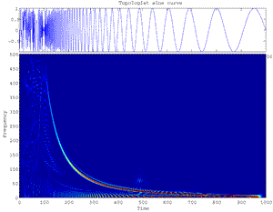
Fig.30 Cohen Time-Frequency Distribution of the Topologist's sine curve.
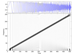
Fig.31 Cohen Time-Frequency Distribution of the signal "linchirp".
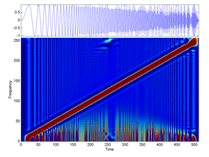
Fig.31b Cohen Time-Frequency Distribution of the signal "linchirp" (jet version).
Fig. Via Wavelab802, for the signal transients
, here are Compared Images of Continuous Wavelet Transforms by using: (a) Gauss, (b) DerGauss, (c) Sombrero, (d) Morlet. (The images are displayed in the Time-Frequency plane).
Fig. The lower-right image (d) of the previous Fig. is enlarged here; The wavelet used is that of Morlet via Wavelab802. One slightly perceives cross structures at high frequencies. (Continuous Wavelet Transform of the signal transients
). (Gray scale version).
Fig.32 Same as above but by using another m-file cwt.m
and displaying parametrization, which is not that of Wavelab802. The cross structures are easier to perceived here. (Image of a Continuous Wavelet Transform of the signal transients
). (Gray scale version).
Fig.33 Same as above but with Colormap Hot
.
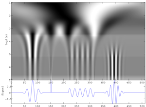
Fig. Image of a Continuous Wavelet Transform of an arbitrary signal that consists of. (1) two slighly different Gabor atoms whose internal frequencies progressively increase, (2) A dirac, (3) A sinusoid, (4) A noise that increases at each sequence repetition.The wavelet is a Sombrero and the wavelet transform uses Wavelab802 version (see also movie)
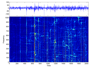
Fig.34 Cohen Time-Frequency Distribution of 2048 Cac40 first-difference daily values (for sigma large).
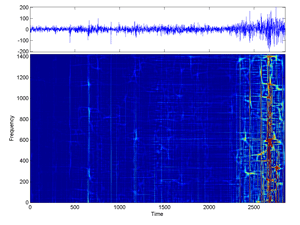
Fig.35 Cohen Time-Frequency Distribution of 2847 Cac40 first-differences (for sigma large).
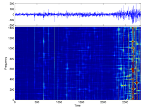
Fig.36 Cohen Time-Frequency Distribution of 2847 Cac40 first-differences daily values (for smaller sigma).