
Complex and Chaotic Nonlinear Dynamics. T.Vialar. Springer. 2009.
Figs. Pictures produced by m-files (or c code).
Some Examples of MATLAB m-files:
PI-M01-M02
| Some Words About: | ||||
|---|---|---|---|---|
| Heading n° | Subject | Documents, or Matlab m-files. | Page | Fig |
| §1.8 §1.9 §1.9.2 |
Bifurcations. In the text hereafter the bifurcations concern singularities with co-dimension greater than 1. | Cusp and Generalized Hopf bifurcations | 39 | |
| Matlab reminders: Matrix powers and exponentials, Eigenvalues, Singular Value Decomposition, Vector and Matrix Norms (m-file): | MatlabMathematicsReminders.m (Reminders that can be skipped). |
|||
1. Each MATLAB m-file group gives an independent simulation.
2. The last m-file (to the right or bottom) of each group runs the simulations.
3. Heading n° indicates the corresponding book sections §.
4. All the MP4-files are embedded in HTML pages.
| PART I - Chap.1 Chap.2 | ||||
|---|---|---|---|---|
| Heading n° | Content | Matlab m-files (or mp4, wmv) | Page | Fig. |
| §1.12 | Elementary example of nonlinear system resolution (m-files): | nonlineareq.m solution.m | 49 | |
| Example of Nonlinear Equations with Jacobian (m-files): | nleqwj.m solveroutine0.m | |||
| Example of Nonlinear Equations with Analytic Jacobian (m-files): | rosenbrockobj.m solveroutine1.m | |||
| §1.7 | Julia Sets (m-files): | JuliaSet.m JuliaSequence.m | 66 | |
| §1.38 §1.35.2 |
Some nonlinear systems: Lorenz, Duffing, Chua circuit, Colpitts oscillator, Rayleigh oscillator, Van der Pol oscillator (for μ=0.2, μ=1, μ=10), and Henon attractor (m-files): |
lorenzeqs.m duffing.m Chua.m Colpitts.m Rayleigh.m vdpeq1.m vdpeq2.m vdpeq3.m henonmap.m attractLIST.m (This file starts the simulations) | 212 191 |
1.33 1.35 |
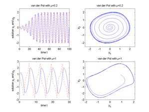
| §1.38 | Plot Van der Pol oscillator for both values μ=0.2, μ=1 (m-files): | vdpeq1.m vdpeq2.m vdpeq3.m vdpSUB.m | 212 | 1.116 |
| §1.38 | Evaluate Van der Pol oscillator for μ varying from 0 to 2 (m-files): | vdpeqMU.m vdpAnim.m [t,(y1,y2)]; [y1, y2] | 212 | 1.116 1.117 1.118 |
| §1.38 | Evaluate Van der Pol oscillator for μ varying from 0 to 2.5. Show [t,y1,y2] (m-files): | vdpeqMU.m vdpAnim3D.m | 212 | 1.118 |
| §1.38 | Movies of previous simulation (mp4.file, wmv-file, 16'): | vdp3D.mp4: 4 movies. (vdp3D.wmv: [t,y1,y2], vdp3D1.wmv : [t,(y1,y2)], vdp3D2.wmv: [y1,y2]) |
212 | 1.116 1.117 1.118 |
| §1.38 | Evaluate Van der Pol oscillator for μ varying from -1.8 to 2.5. [t,y1,y2] (m-files): | vdpeqMU.m vdp3DLong.m | 212 | |
| §1.11.2 | Linear system examples: center, node-sink, spiral-source, 2 saddles (m-files): | Group of five pairs of m-files below: |
44 | |
| - Center (m-files): | center.m centerDyn.m | |||
| - Node-Sink (m-files): | nodesink.m nodesinkDyn.m | |||
| - Spiral Source (m-files): | spiralsource.m spiralsourceDyn.m | |||
| - Saddle 1 (m-files): | saddle1.m saddle1Dyn.m | |||
| - Saddle 2 (m-files): | saddle2.m saddle2Dyn.m | |||
| §1.11.3 | Example of nonlinear system with a (supercritical) Hopf bifurcation (m-files): | 46 | 1.22 | |
| §1.11.3 | Movie of the simulation above (mp4-file, wmv-file, 3'): | 46 | ||
| §1.25 | Example of the restricted three-body problem (m-files): | events.m fct_tbp.m threebodyproblem.m | 196 | |
| §1.35.2.1 | The first example of blue sky orbit underlying catatrophe (Blue Sky Bifurcation, Blue Sky Catastrophe) is the model of N.Gavrilov and A.Shilnikov, 2000 (m-files): | BSCgeneric.m BSCdemoG.m | 192 | 1.103 |
| §1.20 §1.22 §1.26.2 §1.27 |
Torus (genus-1) whose surface is traversed by a point with a regular trajectory (m-files): | TorusPQ.m (see also animation of a genus-1 whose radii change genus1m.mp4) |
72 80 102 103 108 |
1.49 |
| Orbit of a nonlinear system (including Hopf Bifurcation), γ= -1,..,1, μ= -0.5,..,3 (m-file): Attention: Consider as an exercise the question: Is the simulation Dynamic2.mvalid or not? Movie of "Dynamic2" simulation above. Attention: same question as above (mp4-file, wmv-file, 13'): |
Dynamic2.m OrbitDyn2.mp4 (OrbitDyn2.wmv) |
X | ||
| §1.9.21 | Cusp (singularity) Diagram example (m-file): | CuspDiag.m | 39 | X |
| §1.30.1 | Logistic dynamic for alpha=3.5,...,4 (m-files): | logis.m logeqsimu.m | 115 | |
| §1.30.1 | Movie of the basic dynamic (observe the revolution of points) (mp4-file, wmv-file, 1"06'): | logmapDyn.mp4 (logmapDyn.wmv) | 116 | |
| §1.30.3 | Logistic orbit (m-files): | logisticorbit.m | 119 | |
| §1.31.0.2 | Lyapunov Exponent of Logistic orbit (Lce) (m-files): | LyapLog1.m | 128 | |
| §1.31.1 | Iterative maps of logistic equation (m-files): | bosn.m humpdemo.m | 129 | |
| §1.31.6 | 10 iterative maps of logistic equation (m-files): | fct_eqs.m bosses.m | 142 | |
| §1.31.1 | Iterative maps (sliders m-files): | fct_eqs.m inter.m Huslider.m | 129 | |
| Initial values and logistic map (sliders m-files): | logis.m inter1l.m Lslider.m | |||
| §4.1.2 | Logistic map and histogram varying with alpha (m-files): | hyyt.m hylog.m | 336 | |
| §4.1.1 | Spectra, Poincaré sections, histograms of the logistic map for alpha=3.5,..,4 (m-files): | hyyt.m ehsp.m | 331 | |
| §1.37.26 | Power spectrum for alpha=2.6,..,3.6 (m-files): | pppp.m densipp.m pppslid.m | 209 | X |
| §1.37.26 | Movie of the power spectrum for alpha=3.35,..,3.575, lobes (mp4-file, wmv-file, 1"56'): | psd1.mp4 (psd1.wmv) | 209 | X |
| §1.37.26 | Movie of the power spectrum for alpha=3.5,..,4 (mp4-file, wmv-file, 1"05'): | psd2.mp4 (psd2.wmv) | 209 | X |
| Chap.2 | Basic tutorial for the Matlab SVDfunction, i.e. the Singular Value Decomposition (m-file): |
svdEXP.m | 227 | |
| §2.1 | Chaotic Dynamics resulting from Delay model & R.May equation. (Note that in the following m-files, the Matlab svdfunction mentioned above is not directly used). |
(ref. to Medio.1992) | 228 | |
| §2.1 | - 1.Delay model, α=5 (m-files): | medioeq.m medio05.m | 234 | 2.8 2.9 2.10 2.11 |
| §2.1 | - 2.Delay model, α=4.95 (m-files): | medioeq.m medio0495.m | 233 | 2.7 |
| §2.1 | - 3.Delay model, α=4.85 (m-files): | medioeq.m medio0485.m | 233 | 2.6 |
| §2.1 | - 4.Delay model, α=4.75 (m-files): | medioeq.m medio0475.m | 233 | 2.5 |
| §2.1 | - 5.Delay model, α=4.5 (m-files): period-doubling |
medioeq.m medio045.m | 232 | 2.4 |
| §2.1 | - 6.Delay model, α=4.35 (m-files): | medioeq.m medio0435.m | 232 | 2.3 |
| §2.1 | - 7.Delay model, α=4 (m-files): | medioeq.m medio04.m | 232 | 2.2 |
| - 8.Delay model, α=3 (m-files): | medioeq.m medio03.m | |||
| §2.1 | - Dynamic view for alpha varying from 3 to 5 (m-files): | medioeq.m medioanim.m | 228 | 2.2 ↓ 2.10 |
| §2.1 | - Movie of the previous dynamic (mp4-file, wmv-file, 1"39'): | medio.mp4 (medio.wmv) | 228 | 2.2 ↓ 2.10 |
| §2.2.2 | - Attractor reconstructed by using Singular Spectrum Analysis [Delay model & May equation for alpha=5] (m-files): | medioeq.m BT5med.m | 239 | 2.12 |
| §2.2.3 | Singular Spectrum Analysis applied to the cac40 stock-index (2806 daily values, Jan 1988 - April 1998) (m-files): | cac40.m BTcac40.m | 241 | 2.15 |
| §2.3.1 | Histograms of (Pseudo) fractional brownian motion; fBm, 1st and 2nd-difference (sliders m-files): | WhiteNoise.m GenBrownian.m interMB.m MBhslider.m (cf. detrending, nth-difference) | 244 | 2.19 |
| §2.3.1 | Movie of above simulation, loop on H=0.2,..,1 (mp4-file, wmv-file, 53'): | fBM1.mp4 (fBM1.wmv) | 244 | 2.19 |
| §2.3.3 | Simulation of a (pseudo) fract. brownian motion walk in a plane for H=0.5 (m.file): | WhiteNoise.m GenBrownian.m fBmX.m | 250 | 2.21 |
| §2.3.3 | Movie of a bidimensional (pseudo) brownian motion, H=0.53 (mp4-file, wmv-file, 11"): | Walk2D.mp4 (Walk2D.wmv) 11minutes | 252 | 2.21 |
| §2.3.3 | Movie of a (pseudo) 3-dimensional fract. brownian motion, H=0.5 (mp4-file, wmv-file, 11"): | Walk3D.mp4 (Walk3D.wmv) 11minutes | 252 | 2.22 |
PII-S03-S04
| PART II - Chap.3 Chap.4 | ||||
|---|---|---|---|---|
| Heading n° | Content | Matlab m-files (or mp4, wmv) | Page | Fig. |
| §3.4.3 | Generate data of a unidimensional Gaussian distribution, then, plot its normalized histogram estimate and true density (m-files): |
EgaussD.m histpd.m EstimDensity.m | 281 | 3.1 |
| §3.4.3 | Epanechnikov, Biquadratic, Gaussian and Cubic kernels (m-file): |
kernels.m | 280 | X |
| §3.6.1.2 | Gamma (or Euler) function (m-file): | Eugam.m | 301 | 3.5 |
| §4.1 | Poincaré sections, histograms for a stock-index, white noise, logist. map (m-file): |
cac40.m WhiteNoise.m hyyt.m scatplot.m | 331 | X |
| §4.1.2 | Probability Density Function (m-file): | pdf.m | 339 336 |
4.2 |
| §4.1.2 | Natural measure of probability, u-shape convergence (mp4-file, wmv-file, 6'): |
Ushape.mp4 (Ushape.wmv) | 339 | 4.1 4.2 |
PIII-P05-P06
| PART III - Chap.5 Chap.6 | ||||
|---|---|---|---|---|
| Heading n° | Content | Matlab m-files (or mp4, wmv) | Page | Fig. |
| § 5.3 | Fourier Transform example that shows Fourier coefficients in the complex plane, periodicity, periodogram, and power (Years/cycle) (dat-file, m-file): | sunspot.dat FFTperiodicity.m (this file is based on a Matlab.7 demo) | X | |
| Power Spectrum via Periodogram of signal (200Hz) embedded in additive noise (m-file): | periodogramEXP.m (this file is an example of the use of Matlab periodogram.m) | X | ||
| Magnitude and Phase of Transformed Data (m-file): | magphase.m | |||
| § 5.3 | Sum of Wave functions (m-file): | Waves.m | 351 | X |
| § 5.5.1 | Integral of Morlet Wave (m-file): | wavesurf.m | 356 | 5.4 |
| Non-normalized Window (m-file): | arbitrarywindow.m | 371 | 5.13 | |
| § 5.7.4 | Normalized Gauss window (m-file): | gausswindow.m | 371 | |
| § 5.7.4 | Gauss window with its derivative x10² (m-files): | gaussDgauss.m | 371 | 5.13 5.14 |
| § 5.11.1 | Graphs of four window types (m-file): | windows.m | 387 | 5.24 |
| Simultaneous spread variations of a window and a wave function (sliders m-file): | inter32.m gabfon2.m g2slider.m | |||
| Simultaneous translation of a window and a wave function (sliders m-file): | inter3.m gabfonc.m gslider.m | |||
| 2 Gabor functions (or Gabor atoms) (m-file): | gaboret.m | 355 | 5.3 | |
| § 5.7.1 | 1st tutorial about the Matlab convolution function conv(m-file): |
ConvolutionM01.m | ||
| § 5.7.1 | 2nd tutorial about the Matlab convolution function conv(u,v)and convolution matrix function convmtx(b,n)(m-file): |
ConvolutionM02.m Example of convolution matrix for a vector b in the Galois field GF(4), representing the numerator coefficients for a digital filter. |
||
| § 5.7.1 | Schematic representationof the convolution of an arbitrary curve with a sliding wave function (sliders m-files): |
interwav1.m wav1.m wav1slider.m | 368 | 5.11 |
| § 5.7.1 | Movie of previous files (mp4-file, wmv-file, 12'): | Convo.mp4 (Convo.wmv) | 368 | 5.11 |
cwt. cwt1.mused is not a version of Wavelab or Matlab7. Hereafter, The m-file CWT.mused belongs to Wavelab802. |
||||
| § 5.5.3 § 5.17.1 |
Five Gauss-pseudo-wavelet transforms of a stock-index (m-files): Attention: a Gauss-pseudo-wavelet is obviously not a true wavelet in a strict sense (since it does not fulfil the criteria) but allows to point out the wavelet contruction mechanism by means of a useful counterexample. |
cac40.m cwt1.m (*) CACechel.m wtfcacgauss.m(*) (*)Revised on 3 September 2010. |
358 448 449 450 451 452 453 455 456 |
5.6 5.43 5.44 5.45 5.46 5.47 5.48 5.49 |
| § 5.17.1 | Five Morlet wavelet transforms of a stock-index (m-files): | cac40.m cwt1.m CACechel.m wtfcacmorlet.m Revised on 3 September 2010. |
456 455 |
5.48 5.49 X |
| § 5.17 | Image of the Continuous Wavelet Transform of a signal that consists of: (1) two slighly different Gabor atoms whose internal frequencies progressively increase, (2) a Dirac, (3) a sinusoid, (4) and a noise that increases at each repeated sequence. (23') (m-files): |
CWT.m(*) ImageCWT.m(*) CWTanimSig.m (*)m-files belonging to Wavelab802. |
448 449 450 451 452 453 455 456 |
X |
| § 5.17 | Movie of the previous files of the Continous Wavelet Transform. (mp4-file, wmv-file, 23'): | CWTsig.mp4 (CWTsig.wmv) | X | |
| § 5.17 | Display in the Time-Frequency plane, by Wavelab802, for the signal transients, the Compared Images of Continuous Wavelet Transforms by using: (a) Gauss, (b) DerGauss, (c) Sombrero, (d) Morlet. (m-files): |
CWT.m(*) ImageCWT.m(*) CWTtrsComp.m (*)from Wavelab802. |
X | |
| § 5.17 | Display, for the signal transients, the Continuous Wavelet Transforms by using a Morlet wavelet. Image displayed in the Time-Frequency plane.(m-files): |
CWT.m(*) ImageCWT.m(*) CWTtrs.m (*)from Wavelab802. |
X | |
| § 5.10.3 | Example of a spectrogram for the signal transients(m-files): |
transients.asc SpectrogTrans.m | 381 | |
| § 5.18 | Wigner-Ville Time-Frequency Distribution of the signal "transients" (m-files): | wvdist.m transients.asc wgtrans.m (Time-Frequency plane: [0,1] vs. [0,1]) | 456 | X |
| § 5.18 | Wigner-Ville Time-Frequency Distribution of 2 Gabor atoms (m-files): | wvdist.m wg2ats.m (T-F. plane: [0,1] vs. [0,1/2]). | 458 | X |
| § 5.18 | Wigner-Ville Time-Frequency Distribution of 2 slighly different Gabor atoms whose internal frequencies progressively increase (m-files): | wvdist.m wg2atsmv.m (T-F. plane: [0,1] vs. [0,1]). | 458 | X |
| § 5.18 | Movie of above files, observe the (calculation) interference terms (mp4-file, wmv-file, 4'): | WGatoms.mp4 (WGatoms.wmv) (T-F. plane: [0,1] vs. [0,1]). | 458 | X |
| § 5.18 | Same Wigner-Ville Dist. but in the Time-Frequency plane: [0,1] vs. [0,1/2] (m-files): | wvdist.m wg2atsmvHALF.m (T-F. plane: [0,1] vs. [0,1/2]). | 458 | |
| § 5.18 | Movie of the files above (mp4-file, wmv-file, 4'): | WGatomsHALF.mp4 (WGatomsHALF.wmv) | 458 | |
| Alias-Free Generalized Discrete Time-Frequency Distribution of 2 Gabor atoms (m-files): | tfdist.m td2ats.m | X | ||
| § 5.18.1 | Cohen class Time-Frequency Distribution of 2 Gabor atoms (m-files): | ShapeLike.m (5) CohenDist.m Interpol2.m repCH.m |
459 | 5.51 |
| § 5.18.1 | Cohen class Time-Frequency Distribution of 2 slighly different Gabor atoms whose internal frequencies progressively increase (m-files): | ShapeLike.m CohenDist.m Interpol2.m repCHmv.m | 459 | X |
| § 5.18.1 | Movie of the previous files of the Cohen class Time-Frequency Dist. (mp4-file, wmv-file, 4'): | ChGatoms.mp4 (ChGatoms.wmv compare with its spectrogram: SpectgAts.mp4) | 459 | X |
| Comparison of Representations In the Time-Frequency Plane: a) Cohen Dist. b) Wigner-Ville Dist., c) Spectrogam. for a same basic signal consisting of: two slighly different Gabor atoms whose internal frequencies progressively increase. (4'). |
COMPsigBasic.html(*) (*)Page including 4 mp4 animations. |
|||
| § 5.18.1 | Cohen class Time-Frequency Distribution of a signal that consists of: (1) two slighly different Gabor atoms whose internal frequencies progressively increase, (2) a Dirac, (3) a sinusoid, (4) and a noise that increases at each repeated sequence. (23') (m-files): | ShapeLike.m CohenDist.m Interpol2.m CHMultSig.m(*) (*)Revised on 3 september 2010. |
461 | X |
| § 5.18.1 | Movie of the previous files of the Cohen class Time-Frequency Dist. (mp4-file, wmv-file, 4'): | CHsignals.mp4 (CHsignals.wmv) (compare with its Wigner-Ville dist.: WIGsignalsFULL.mp4 (WIGsignalsFULL.wmv) (T-F plane [0,1] vs. [0,1]) WIGsignalsHALF.mp4 (WIGsignalsHALF.wmv) ([0,1] vs. [0,1/2]). See interference terms. | X X |
|
| Comparison of Representations In the Time-Frequency Plane: a) Cohen Dist. b) Wigner-Ville Dist., c) Continuous Wavelet Transf. for a same signal consisting of: (1) two slighly different Gabor atoms whose internal frequencies progressively increase, (2) a Dirac, (3) a sinusoid, (4) and a noise that increases at each repeated sequence. (23'). |
COMPsig.html(*) (*)Page including 4 mp4-animations. |
|||
| § 5.18.1 | Cohen class Time-Frequency Distribution of the signal "transients" (m-files): | ShapeLike.m CohenDist.m Interpol2.m transients.asc ConhenDisttransients.m | X | |
| § 5.18.1 | Cohen class Time-Frequency Distribution of the topologist's sine curve (m-files): | ShapeLike.m CohenDist.m Interpol2.m topoCH.m | X | |
| § 5.18.1 | Cohen class Time-Frequency Distribution of the signal "linchirp" (m-files): | ShapeLike.m CohenDist.m Interpol2.m linchirp.asc ConhenDistlinchirp.m | X | |
| § 5.18.1 | Cohen class Time-Frequency Distribution of 2048 Data of cac40 1st-differences (m-files): | ShapeLike.m CohenDist.m Interpol2.m cac40.m ConhenDistCAC.m | X | |
| § 5.18.1 | Cohen class Time-Frequency Distribution of 2847 Data of cac40 1st-differences (m-files): | Cohen class Time-Frequency Distribution of 2847 Data of cac40 1st-differences (m-files): ShapeLike.m CohenDist.m Interpol2.m cac40.m ConhenDistCAC2847.m | X | |
| § 5.18.1 | List of classic signals available as asc files (or via txt-files): - transients info.txt, - linchirp, - tweet, - sunspots, - greasy, - caruso info.txt, - HochNMR info.txt, - RaphNMR info.txt, - esca info.txt. |
transients.asc (or via transients.txt) linchirp.asc (or via linchirp.txt) tweet.asc (or via tweet.txt) sunspots.asc (or via sunspots.txt) greasy.asc (or via greasy.txt) caruso.asc (or via caruso.txt) HochNMR.asc (or via HochNMR.txt) RaphNMR.asc (or via RaphNMR.txt) esca.asc (or via esca.txt) |
||
| § 5.18.1 | Plot these signals in only one picture of nine subplots (m-file): | Signals9.m (demo using the above asc signals) | X | |
| § 5.18.1 | Plot individually each one of the above signals: (m-files): | sg1plot.m (transients) sg2plot.m (linchirp) sg3plot.m (tweet) sg4plot.m (sunspots) sg5plot.m (greasy) sg6plot.m (caruso) sg7plot.m (HochNMR) sg8plot.m (RaphNMR) sg9plot.m (esca) |
X X X X X X X X X |
|
| Plot in only one picture the nine first-return map subplots of each one of previous signals (asc-files, m-files) | transients.asc linchirp.asc tweet.asc sunspots.asc greasy.asc caruso.asc HochNMR.asc RaphNMR.asc esca.asc FRMSignals.m (demo) |
X | ||
| § 5.18.1 | Cohen class Time-Frequency Distribution of the signal greasyanalyzed on a segment of 512 data scrolling point-by- point along the entire signal made of 8192 data. Each sample is resized (m-files) |
greasy.asc ShapeLike.m CohenDist.m Interpol2.m CohenGREASYanim.m 6 minutes 30 s |
X | |
| § 5.18.1 | Movie of the above m-files (mp4-file - embedded in html page, and wmv file): |
greasyCH.mp4 6 minutes 30s (greasyCH.wmv Mid-resolution, 36Mo) |
X X |
|
| § 5.18.1 | Cohen class Time-Frequency Distribution of the signal tweetanalyzed on a segment of 512 data scrolling point-by- point along the entire signal made of 8192 data. Each sample is resized (m-files) |
tweet.asc ShapeLike.m CohenDist.m Interpol2.m CohenTWEETanim.m 8 minutes 32 s |
X | |
| § 5.18.1 | Movie of the above animation (mp4, wmv files): |
tweetCH.mp4 8 minutes 32s (tweetCH.wmv Mid-resolution, 66Mo) |
X X |
|
| § 5.18.1 | Cohen class Time-Frequency Distribution of the signal tweetanalyzed on a shorter segment of 256 data scrolling point-by-point along the entire signal made of 8192 data. Each sample is resized (m-files) |
tweet.asc ShapeLike.m CohenDist.m Interpol2.m CohenTWEETanim256.m | ||
| § 5.18.1 | Movie of the above animation (mp4, wmv files): | tweet256CH.mp4 8 minutes 49s (tweet256CH.wmv Mid-resolution, 51Mo) |
||
| § 5.18.1 | Cohen class Time-Frequency Distribution of the signal Carusoanalyzed on a segment of 512 data scrolling point-by- point along the entire signal formed of 50.000 data. Each sample is resized (m-files): |
caruso.asc ShapeLike.m CohenDist.m Interpol2.m CohenCARUSOanim.m 36 minutes 47 s |
X | |
| § 5.18.1 | Movie of the above animation (mp4, wmv files): |
carusoCH.mp4 36 minutes 47s (carusoCH.wmv Mid-resolution, 208Mo) |
X X |
|
| § 5.18.1 | Display together the Cohen Distributions of the long signals above: tweet, greasy, Caruso (mp4 files): | CHlongSigs.html This page may be slow to display (∑≈230Mo). |
||
| Matching Pursuit by using Wavelab802: | ||||
|---|---|---|---|---|
| Heading n° | Content | Zip-files of Matlab m-files |
Page | Fig |
| §6.2.1 | 1a. Example of animation of an Atomic Decomposition into Cosine Packets by Matching Pursuit of the signal Linchirp, 512 data. (zip-file): |
|
495 496 497 |
X |
| §6.2.2 | 1b. Example of animation of an Atomic Decomposition into Wavelet Packets by Matching Pursuit of the signal Linchirp, 512 data. (zip-file): |
|
497 498 499 |
X |
| §5.14.5 | 2a. A Demo of Matching Pursuit applied to the signal transients, which displays: 1. Cosine Packet Synthesis Table; 2. Cosine Pack. Residuals Table; 3. Compression Numbers; 4. Phase plane. (zip-file): |
|
424 426 |
X X |
| §5.14.5 | 2b. A Demo of Matching Pursuit applied to the signal transients, which displays: 1. Wavelet Packet Synthesis Table; 2. Wavelet Packet Residuals Table; 3. Compression Numbers; 4. Phase plane. (zip-file) |
424 426 |
X X |
|
5. In PIII-P05-P06 above the file ShapeLike.m was missing, it has been added.
6. For now, the Mallat & Zhang version of the Matching Pursuit Algorithm (i.e. time-frequency atom dictionaries, or stochastic atom dictionaries..) is not shown here.
PIV-E07-E08
| PART IV - Chap.7 Chap.8 | ||||
|---|---|---|---|---|
| Heading n° | Content | Matlab m-files (or mp4, wmv) | Page | Fig. |
| §7.3.2 | Reminders about Cobb-Douglas and CES production functions: | Production fcts. or via pdf file | 532 540 564 603 |
|
| §7.3 | Reference Solow Model (1956) and Steady State (m-files): | ces.m cobbdouglas.m Vest.m netVest.m TnestVest2.m SolowR.m | 531 532 |
X |
| §7.3.2 | Animation of Solow Model (1956) when the savings rate s varies (sliders, m-files): | cobbdouglas.m VestCB.m netVestCB.m TnestVestCB.m SolowSUB.m SwSLID.m | 531 | X |
| §7.3.2 | Movie of previous files (mp4-file, wmv-file, 08'): | slw.mp4 (slw.wmv) | 531 | X |
| §7.12 | Some words about: | Goodwin Model (1967) | 592 | |
| §7.12 | Goodwin Model (1967) (m-files): | goodwin.m good1sim.m | 592 | |
| §7.12 | Goodwin Model (1990) (m-files): | goodwin2.m good2sim.m | 592 | |
1.Each MATLAB m-file group gives an independent simulation.
2. The last m-file (to the right or bottom) of each group runs the simulations.
3. Heading n° indicates the corresponding book sections §.
4. All the MP4-files are embedded in HTML pages.
5. In PIII-P05-P06 above the file
ShapeLike.mwas missing, it has been added.
6. For now, the Mallat & Zhang versions of the Matching Pursuit Algorithm (i.e. time-frequency atom dictionaries, or stochastic atom dictionaries.. ) is not shown here.
7.Some m-files use syntaxes developed via versions anterior to Matlab.7.0. R14.
8.This material is only intented for didactic uses.
Examples of movie (menu): views
Views of each animation MP4 web page
- Reach mp4 files to save as target ..
- Reach wmv files to save as target ..
Revised on January 13, 2020.